Youth Risk Behavior Surveillance

Youth Risk Behavior Surveillance
Every two years, the Centers for Disease Control and Prevention conduct the Youth Risk Behavior Surveillance System (YRBSS) survey, where it takes data from high schoolers (9th through 12th grade), to analyze health patterns.
Load the data
data(yrbss)
glimpse(yrbss)
## Rows: 13,583
## Columns: 13
## $ age <int> 14, 14, 15, 15, 15, 15, 15, 14, 15, 15, 15, 1…
## $ gender <chr> "female", "female", "female", "female", "fema…
## $ grade <chr> "9", "9", "9", "9", "9", "9", "9", "9", "9", …
## $ hispanic <chr> "not", "not", "hispanic", "not", "not", "not"…
## $ race <chr> "Black or African American", "Black or Africa…
## $ height <dbl> NA, NA, 1.73, 1.60, 1.50, 1.57, 1.65, 1.88, 1…
## $ weight <dbl> NA, NA, 84.4, 55.8, 46.7, 67.1, 131.5, 71.2, …
## $ helmet_12m <chr> "never", "never", "never", "never", "did not …
## $ text_while_driving_30d <chr> "0", NA, "30", "0", "did not drive", "did not…
## $ physically_active_7d <int> 4, 2, 7, 0, 2, 1, 4, 4, 5, 0, 0, 0, 4, 7, 7, …
## $ hours_tv_per_school_day <chr> "5+", "5+", "5+", "2", "3", "5+", "5+", "5+",…
## $ strength_training_7d <int> 0, 0, 0, 0, 1, 0, 2, 0, 3, 0, 3, 0, 0, 7, 7, …
## $ school_night_hours_sleep <chr> "8", "6", "<5", "6", "9", "8", "9", "6", "<5"…Exploratory Data Analysis on Weight
skim(yrbss) #count number of NAs in weight - 1004; summary statistics| Name | yrbss |
| Number of rows | 13583 |
| Number of columns | 13 |
| _______________________ | |
| Column type frequency: | |
| character | 8 |
| numeric | 5 |
| ________________________ | |
| Group variables | None |
Variable type: character
| skim_variable | n_missing | complete_rate | min | max | empty | n_unique | whitespace |
|---|---|---|---|---|---|---|---|
| gender | 12 | 1.00 | 4 | 6 | 0 | 2 | 0 |
| grade | 79 | 0.99 | 1 | 5 | 0 | 5 | 0 |
| hispanic | 231 | 0.98 | 3 | 8 | 0 | 2 | 0 |
| race | 2805 | 0.79 | 5 | 41 | 0 | 5 | 0 |
| helmet_12m | 311 | 0.98 | 5 | 12 | 0 | 6 | 0 |
| text_while_driving_30d | 918 | 0.93 | 1 | 13 | 0 | 8 | 0 |
| hours_tv_per_school_day | 338 | 0.98 | 1 | 12 | 0 | 7 | 0 |
| school_night_hours_sleep | 1248 | 0.91 | 1 | 3 | 0 | 7 | 0 |
Variable type: numeric
| skim_variable | n_missing | complete_rate | mean | sd | p0 | p25 | p50 | p75 | p100 | hist |
|---|---|---|---|---|---|---|---|---|---|---|
| age | 77 | 0.99 | 16.16 | 1.26 | 12.00 | 15.0 | 16.00 | 17.00 | 18.00 | ▁▂▅▅▇ |
| height | 1004 | 0.93 | 1.69 | 0.10 | 1.27 | 1.6 | 1.68 | 1.78 | 2.11 | ▁▅▇▃▁ |
| weight | 1004 | 0.93 | 67.91 | 16.90 | 29.94 | 56.2 | 64.41 | 76.20 | 180.99 | ▆▇▂▁▁ |
| physically_active_7d | 273 | 0.98 | 3.90 | 2.56 | 0.00 | 2.0 | 4.00 | 7.00 | 7.00 | ▆▂▅▃▇ |
| strength_training_7d | 1176 | 0.91 | 2.95 | 2.58 | 0.00 | 0.0 | 3.00 | 5.00 | 7.00 | ▇▂▅▂▅ |
yrbss %>%
  ggplot(aes(x = weight)) +
    geom_density() +
    theme_bw() +
    labs(title = "Distribution of Youth Weight",
         x = "Weight",
         y = "Density")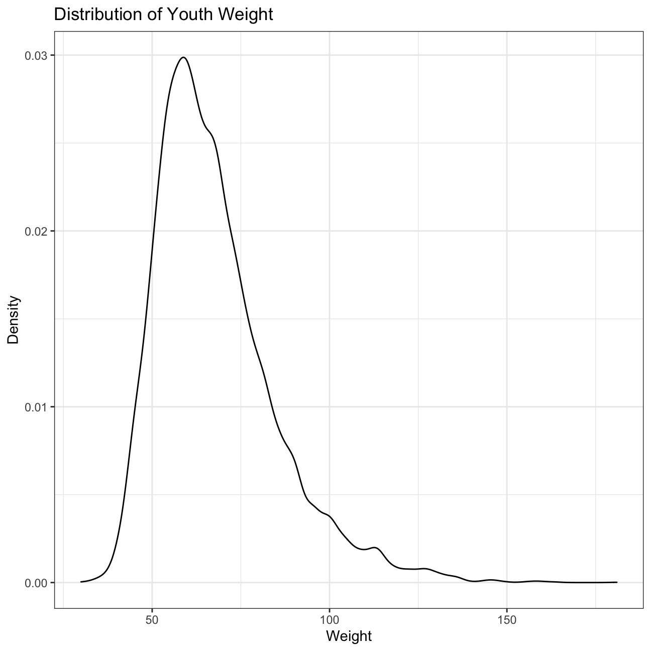
# Youth weight looks relatively right-skewed, meaning that more youth are to the left of the weight distribution.Relationship between weight and physical activity level
# Create indicator for activity level
yrbss <- yrbss %>%
  mutate(physical_3plus = ifelse(physically_active_7d >= 3, "yes", "no"))

#Count number of individuals active versus not active using count
count <- yrbss %>%
  count(physical_3plus) %>%
  mutate(percentage = n/sum(n) * 100)

count
## # A tibble: 3 × 3
## physical_3plus n percentage
## <chr> <int> <dbl>
## 1 no 4404 32.4
## 2 yes 8906 65.6
## 3 <NA> 273 2.01#Count number of individuals active versus not active using group_by & summarise
group_by <- yrbss %>%
group_by(physical_3plus) %>%
summarise(count = n()) %>%
mutate(percentage = count/sum(count) * 100)
group_by## # A tibble: 3 × 3
## physical_3plus count percentage
## <chr> <int> <dbl>
## 1 no 4404 32.4
## 2 yes 8906 65.6
## 3 <NA> 273 2.01# There are almost half of individuals as active individuals who are less active. There is also NAs in level of activity in this dataset.95% confidence interval - proportion of youth who are not active
prop.test(x = 4404, # number of high schoolers who exercise fewer than 3 days a week
          n = 13583, # number of total trials
          p = 0.5, #null hypothesis being that the proportion of population of activity levels equal
          alternative = "two.sided", # two-tailed alternative hypothesis
          conf.level = 0.95, # 95% confidence internal assuming normal distribution
          correct = F)
##
## 1-sample proportions test without continuity correction
##
## data: 4404 out of 13583
## X-squared = 1679, df = 1, p-value <2e-16
## alternative hypothesis: true p is not equal to 0.5
## 95 percent confidence interval:
## 0.316 0.332
## sample estimates:
## p
## 0.324# Confidence interval = (0.316, 0.332)Compare subgroup relationships between activity level and weight
yrbss %>%
  filter(!is.na(physical_3plus)) %>%
  ggplot(aes(x = physical_3plus, y = weight)) +
  geom_boxplot() +
  labs(title = "Boxplot of weights for different activity levels",
       x = "Activity level",
       y = "Weight") +
  NULL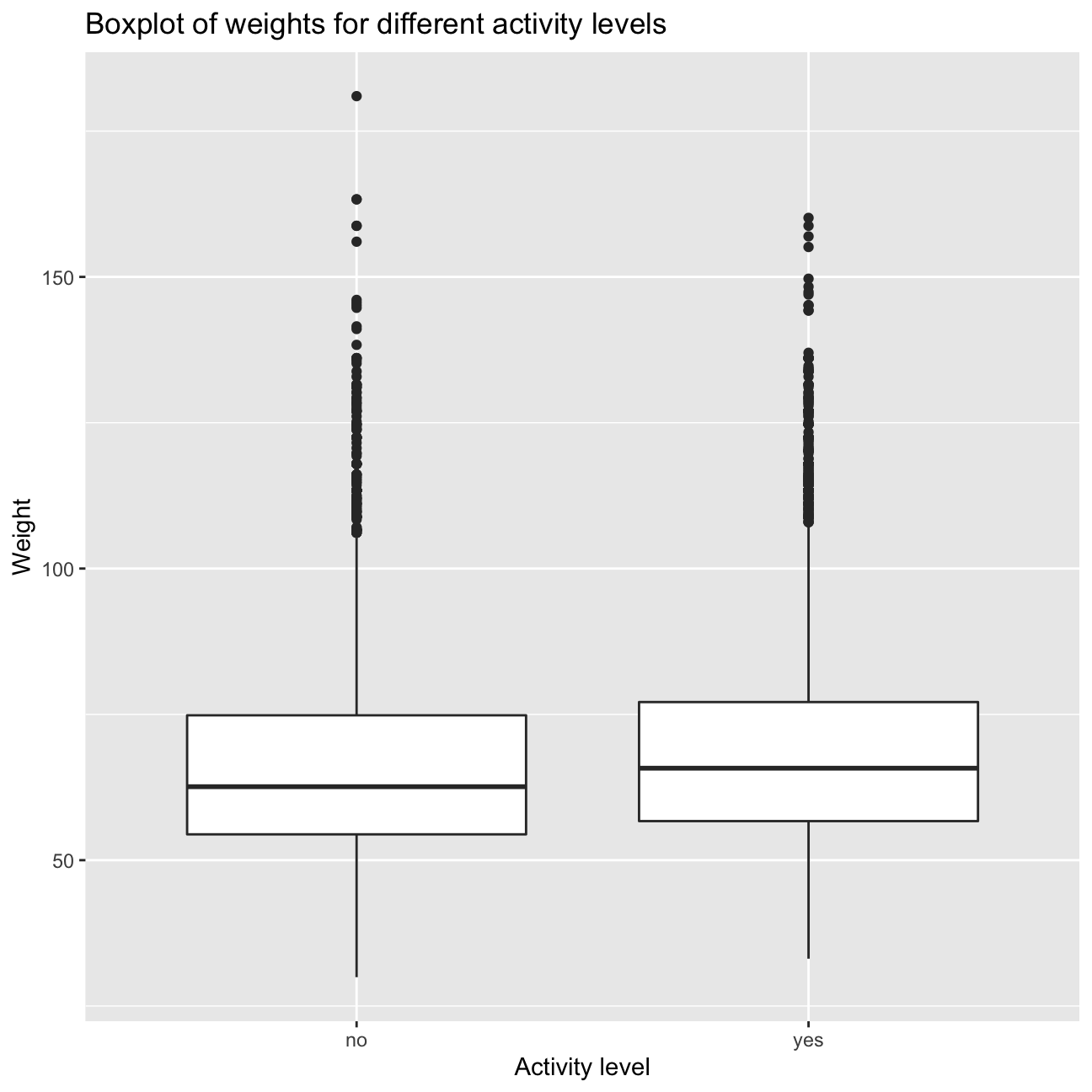
# Graphically, the medians of these two variables don't look too different and the IQR either, implying that, weights do not differ depending on activity level. However, there are many outliers in both active and non-active groups. Confidence Intervals - 1-sample by level of activity
#Calculate summary statistics
ci_using_formulas <- yrbss %>%
  select(weight, physical_3plus) %>%
  filter(!is.na(physical_3plus)) %>%
  group_by(physical_3plus) %>%
  summarise(mean = mean(weight, na.rm = TRUE),
            sd = sd(weight, na.rm = TRUE),
            count = n(),
            se = sd / sqrt(count),
            t = qt(0.975, count-1),
            margin = t*se,
            l_ci = mean - margin,
            h_ci = mean + margin)

 ci_using_formulas
## # A tibble: 2 × 9
## physical_3plus mean sd count se t margin l_ci h_ci
## <chr> <dbl> <dbl> <int> <dbl> <dbl> <dbl> <dbl> <dbl>
## 1 no 66.7 17.6 4404 0.266 1.96 0.521 66.2 67.2
## 2 yes 68.4 16.5 8906 0.175 1.96 0.342 68.1 68.8# Confidence interval for not active: (66.2, 67.2)
# Confidence interval for active: (68.1, 68.8)
# The confidence intervals do not overlap, and the difference should be at least 95% statistically significant.Difference in mean hypothesis test with formula & infer
Null hypothesis: mean weights are the same for those who exercise at least 3 times a week, and those who don’t Alternative hypothesis: mean weights are different for those who exercise at least 3 times a week, and those who don’t
Test using formula:
t.test(weight ~ physical_3plus,
       alternative = "two.sided",
       conf.level = 0.95,
       data = yrbss)
##
## Welch Two Sample t-test
##
## data: weight by physical_3plus
## t = -5, df = 7479, p-value = 9e-08
## alternative hypothesis: true difference in means between group no and group yes is not equal to 0
## 95 percent confidence interval:
## -2.42 -1.12
## sample estimates:
## mean in group no mean in group yes
## 66.7 68.4# p-value very small, hence very statistically significant. We reject the null hypothesis and that there is evidence to show that there is difference in mean between those who exercise at least 3 times a week, and those who don't.Testing using infer:
Initialise the test by calculating the means in this sample.
obs_diff <- yrbss %>%
  filter(!is.na(physical_3plus)) %>% # filter so that there are no NAs
  specify(weight ~ physical_3plus) %>%
  calculate(stat = "diff in means", order = c("yes", "no"))

obs_diff #1.77 difference in means in this sample
## Response: weight (numeric)
## Explanatory: physical_3plus (factor)
## # A tibble: 1 × 1
## stat
## <dbl>
## 1 1.77Simulate the null hypothesis using infer
set.seed(1234)

null_dist <- yrbss %>%
  filter(!is.na(physical_3plus)) %>%
  # specify variables
  specify(weight ~ physical_3plus) %>%

  # assume independence, i.e, there is no difference
  hypothesize(null = "independence") %>%

  # generate 1000 reps, of type "permute"
  generate(reps = 1000, type = "permute") %>%

  # calculate statistic of difference, namely "diff in means"
  calculate(stat = "diff in means", order = c("yes", "no"))
Visualise and plot hypothesis testing:
ggplot(data = null_dist, aes(x = stat)) +
geom_histogram() 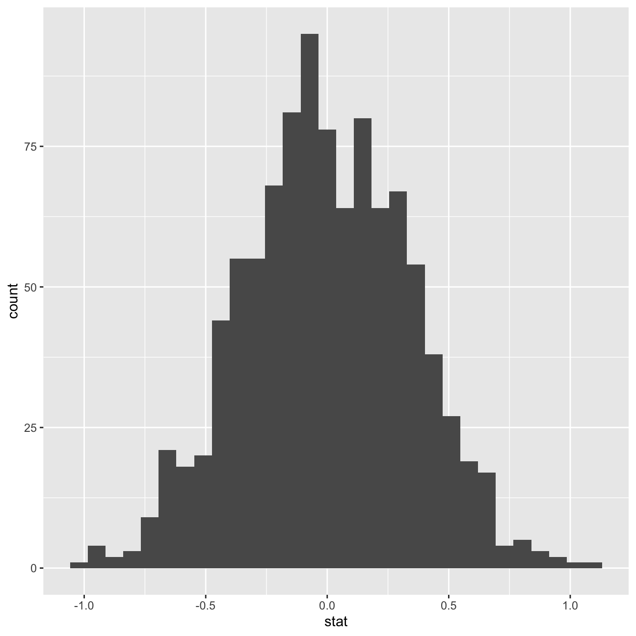
null_dist %>% visualize() +
  shade_p_value(obs_stat = obs_diff, direction = "two-sided")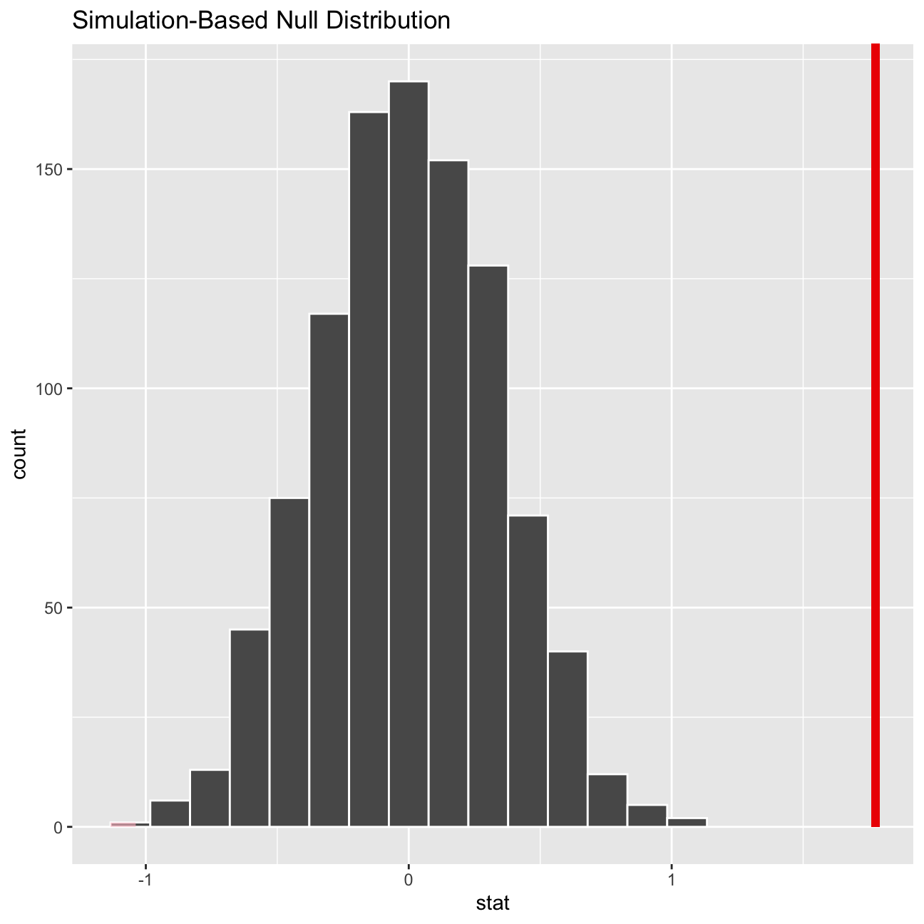
null_dist %>%
  get_p_value(obs_stat = obs_diff, direction = "two_sided")
## # A tibble: 1 × 1
## p_value
## <dbl>
## 1 0