Analysis of Rent in Bay Area

Rents in San Francsisco 2000-2018
Data dictionary:
| variable | class | description |
|---|---|---|
| post_id | character | Unique ID |
| date | double | date |
| year | double | year |
| nhood | character | neighborhood |
| city | character | city |
| county | character | county |
| price | double | price in USD |
| beds | double | n of beds |
| baths | double | n of baths |
| sqft | double | square feet of rental |
| room_in_apt | double | room in apartment |
| address | character | address |
| lat | double | latitude |
| lon | double | longitude |
| title | character | title of listing |
| descr | character | description |
| details | character | additional details |
The dataset was used in a recent tidyTuesday project.
# download directly off tidytuesdaygithub repo

rent <- readr::read_csv('https://raw.githubusercontent.com/rfordatascience/tidytuesday/master/data/2022/2022-07-05/rent.csv')skimr::skim(rent)| Name | rent |
| Number of rows | 200796 |
| Number of columns | 17 |
| _______________________ | |
| Column type frequency: | |
| character | 8 |
| numeric | 9 |
| ________________________ | |
| Group variables | None |
Variable type: character
| skim_variable | n_missing | complete_rate | min | max | empty | n_unique | whitespace |
|---|---|---|---|---|---|---|---|
| post_id | 0 | 1.00 | 9 | 14 | 0 | 200796 | 0 |
| nhood | 0 | 1.00 | 4 | 43 | 0 | 167 | 0 |
| city | 0 | 1.00 | 5 | 19 | 0 | 104 | 0 |
| county | 1394 | 0.99 | 4 | 13 | 0 | 10 | 0 |
| address | 196888 | 0.02 | 1 | 38 | 0 | 2869 | 0 |
| title | 2517 | 0.99 | 2 | 298 | 0 | 184961 | 0 |
| descr | 197542 | 0.02 | 13 | 16975 | 0 | 3025 | 0 |
| details | 192780 | 0.04 | 4 | 595 | 0 | 7667 | 0 |
Variable type: numeric
| skim_variable | n_missing | complete_rate | mean | sd | p0 | p25 | p50 | p75 | p100 | hist |
|---|---|---|---|---|---|---|---|---|---|---|
| date | 0 | 1.00 | 2.01e+07 | 44694.07 | 2.00e+07 | 2.01e+07 | 2.01e+07 | 2.01e+07 | 2.02e+07 | ▁▇▁▆▃ |
| year | 0 | 1.00 | 2.01e+03 | 4.48 | 2.00e+03 | 2.00e+03 | 2.01e+03 | 2.01e+03 | 2.02e+03 | ▁▇▁▆▃ |
| price | 0 | 1.00 | 2.14e+03 | 1427.75 | 2.20e+02 | 1.30e+03 | 1.80e+03 | 2.50e+03 | 4.00e+04 | ▇▁▁▁▁ |
| beds | 6608 | 0.97 | 1.89e+00 | 1.08 | 0.00e+00 | 1.00e+00 | 2.00e+00 | 3.00e+00 | 1.20e+01 | ▇▂▁▁▁ |
| baths | 158121 | 0.21 | 1.68e+00 | 0.69 | 1.00e+00 | 1.00e+00 | 2.00e+00 | 2.00e+00 | 8.00e+00 | ▇▁▁▁▁ |
| sqft | 136117 | 0.32 | 1.20e+03 | 5000.22 | 8.00e+01 | 7.50e+02 | 1.00e+03 | 1.36e+03 | 9.00e+05 | ▇▁▁▁▁ |
| room_in_apt | 0 | 1.00 | 0.00e+00 | 0.04 | 0.00e+00 | 0.00e+00 | 0.00e+00 | 0.00e+00 | 1.00e+00 | ▇▁▁▁▁ |
| lat | 193145 | 0.04 | 3.77e+01 | 0.35 | 3.36e+01 | 3.74e+01 | 3.78e+01 | 3.78e+01 | 4.04e+01 | ▁▁▅▇▁ |
| lon | 196484 | 0.02 | -1.22e+02 | 0.78 | -1.23e+02 | -1.22e+02 | -1.22e+02 | -1.22e+02 | -7.42e+01 | ▇▁▁▁▁ |
#The variable types are primarily of numeric and character data type. The character variable 'descr' has the most missing values (197542 observations being NA) followed by the variables 'address', 'lon','lat',and 'details'. All categorical variables are of character type and numeric variables (except date and year) correspond to numeric data type.Plot of the top 20 cities in terms of % of classifieds between 2000-2018.
# Filter original dataset and produce new dataset containing classifieds
top_cities <- rent %>%
  filter(year %in% c(2000:2018)) %>%
  count(city) %>%
  mutate(city_listing = n) %>%
  mutate(classifieds = city_listing / sum(city_listing) * 100)

# Plotting bar chart using top_cities dataset
top_cities %>%
  slice_max(order_by = classifieds, n = 20) %>%
  ggplot(aes(x = classifieds, y = fct_reorder(city, classifieds))) +
  geom_col() +
  theme_minimal()+
  labs( title="San Francisco accounts for more than a quarter of all rental classfields",subtitle="% of Craiglist listings, 2000-2018",x = NULL,y=NULL,caption = "Source:Pennington, Kate (2018). Bay Area Craigslist Rental Housing Posts, 2000-2018" )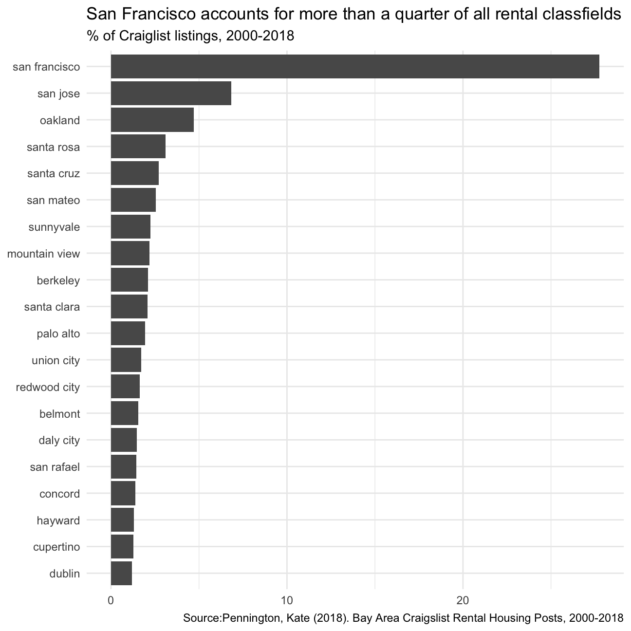
Plot of the evolution of median prices in San Francisco for 0, 1, 2, and 3 bedrooms listings. The final graph should look like this
# Filter dataset, produce median prices, and plot line graph facetted by number of beds
 sf_median_prices<-rent %>%
  filter(city=="san francisco" & beds %in% c(0:3)) %>%
  group_by(beds,year) %>%
  summarize(med = median(price))%>%
   ggplot(aes(x=year,y=med,color=factor(beds))) + geom_line() +
  facet_grid(~beds)+
  labs( title="San Francisco rents have been steadily increasing",subtitle="0 to 3-bed listings,2000-2018",x = NULL,y=NULL,caption = "Source:Pennington, Kate (2018). Bay Area Craigslist Rental Housing Posts, 2000-2018" )+
   theme_bw()+
   theme(legend.position="none")

 # Display graph
 sf_median_prices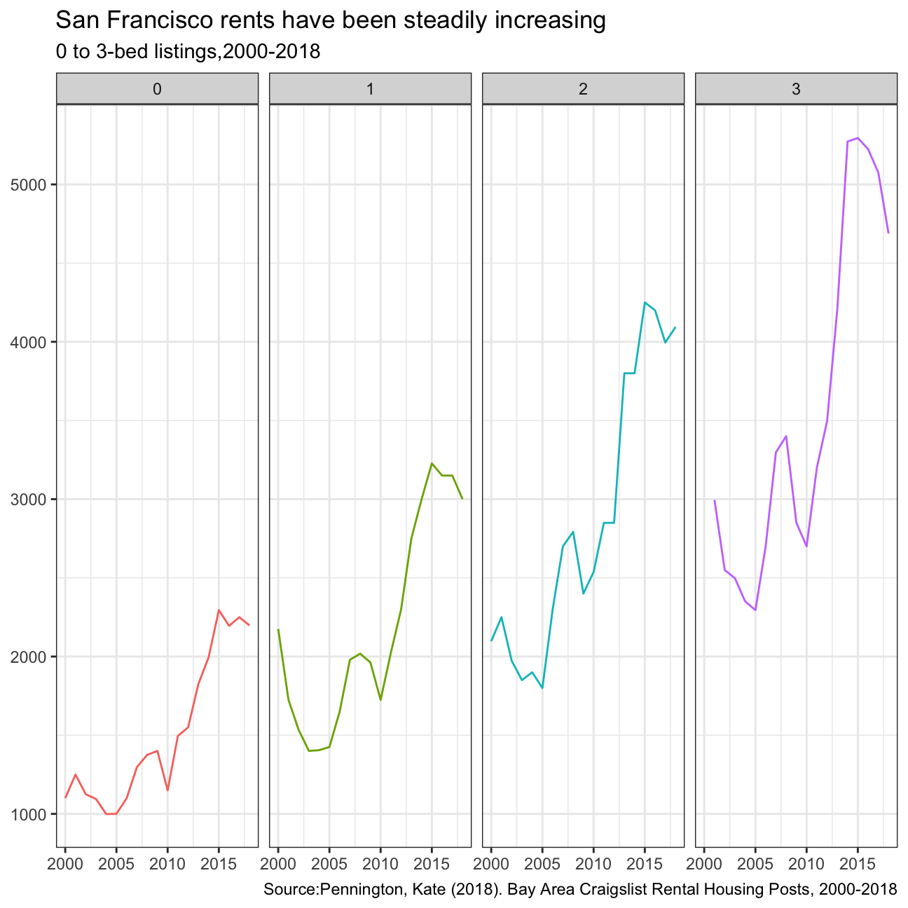
Plot of median rental prices for the top 12 cities in the Bay area.
# Filter original dataset, find median prices of selected cities, and plot
spirit_plot<-rent %>%
  filter(city %in% c("san francisco","oakland","san jose","berkeley","santa cruz","santa rosa","mountain view","san mateo","palo alto","santa clara","union city","sunnyvale") & beds==1) %>%
  group_by(city,year) %>%
  summarize(med = median(price))%>%
  ggplot(aes(x=year,y=med, color = factor(city))) +
  geom_line() +
  facet_wrap(~city)+
  labs( title="Rental prices for 1-bedroom flats in the Bay Area",x = NULL,y=NULL,caption = "Source:Pennington, Kate (2018). Bay Area Craigslist Rental Housing Posts, 2000-2018" )+
  theme_bw()+
  theme(legend.position="none")

# Display plot
spirit_plot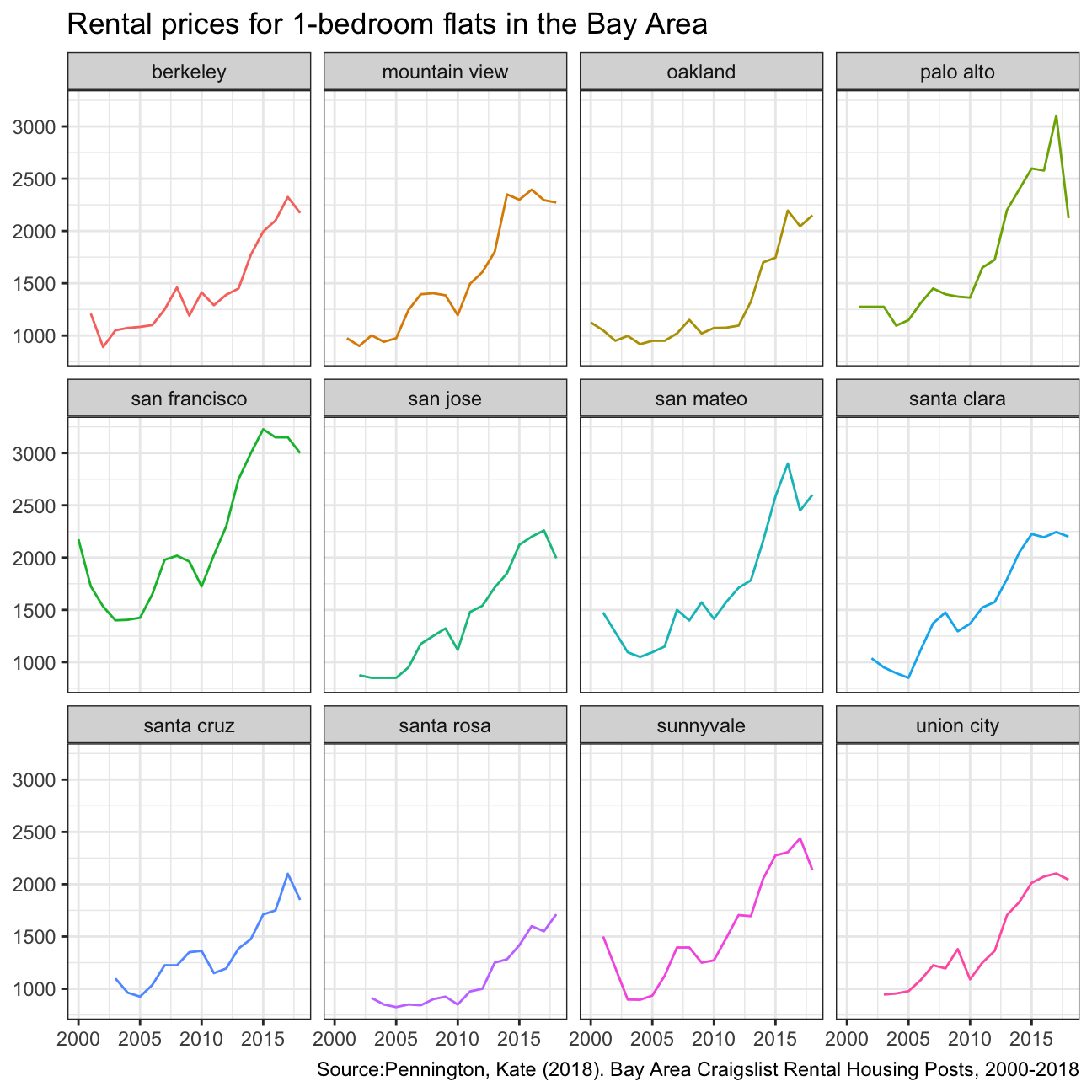
San Francisco is the city that has the highest percentages of rental listings between the years 2000 and 2018, falling just under 30% of total listings. Average prices of all common types of listings (between 0 and 3 bedrooms) took a hit during and after the financial crisis in 2008, and saw prices surge to more than double its pre-pandemic high in 2018, despite it levelling off post-2015. Many cities in the same Bay area saw a similar surge of rental prices for a 1-bedroom apartment, mainly for job-seekers.
The surge in rental prices may be caused by high housing prices in San Francisco. Purchasing a house and renting a house act as (somewhat perfect) substitutes, diverting job-seekers’ demand for houses towards rental houses. Seeing an opportunity, house-owners may be more willing to supply their houses in the rental market, hence seeing an increase in supply of rental houses. 2 and more bedroom rentals also saw prices rising, which may indicate not only job-seekers, but also families are priced out of purchasing a house, but supply has fallen far behind to soak up the increase in demand.