Plotting Information

Plotting data using a time-series scatterplot with a trendline.

tidyweather <- tidyweather %>%
  mutate(date = ymd(paste(as.character(Year), Month, "1")),
         month = month(date, label=TRUE),
         year = year(date))

ggplot(tidyweather, aes(x=date, y = delta))+
  geom_point()+
  geom_smooth(color="red") +
  theme_bw() +
  labs (
    title = "Weather Anomalies",
    x = "Year",
    y = "Temperature deviaton",
    caption = "Source: https://data.giss.nasa.gov/gistemp/tabledata_v4/NH.Ts+dSST.txt"
  ) +
  NULL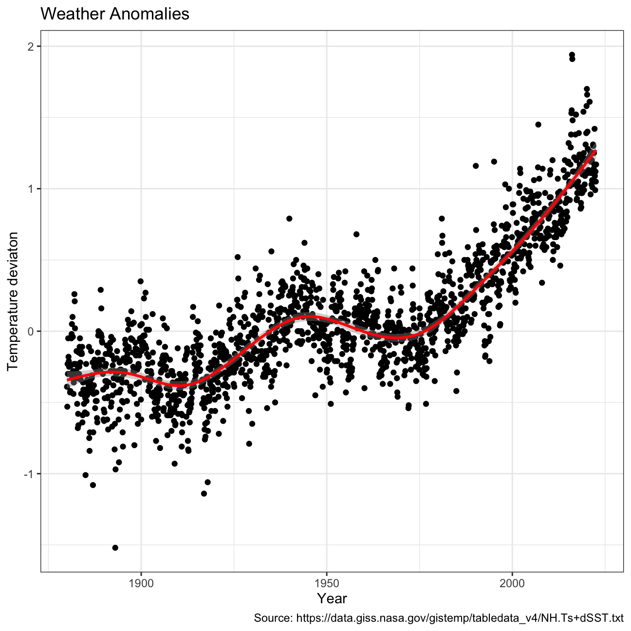

Producing a scatter plot showing the temperature anomalies by month.

ggplot(tidyweather, aes(x=date, y = delta))+
  geom_point()+
  geom_smooth(color="red") +
  theme_bw() +
  labs (
    title = "Weather Anomalies",
    x = "Year",
    y = "Temperature deviaton",
    caption = "Source: https://data.giss.nasa.gov/gistemp/tabledata_v4/NH.Ts+dSST.txt"
  ) +
  facet_wrap(~month) +
  NULL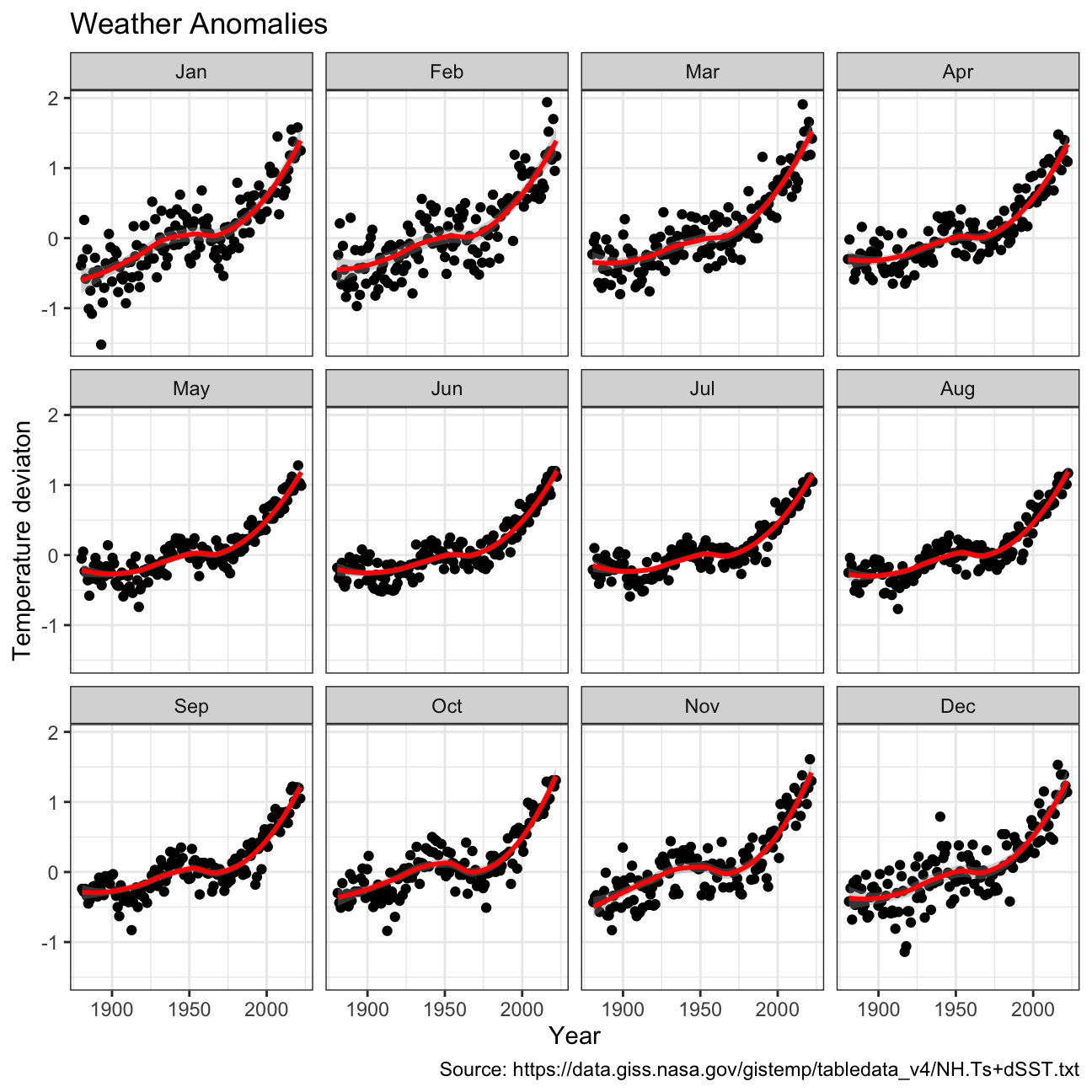

Grouping data into different time periods to study historical data.

comparison <- tidyweather %>% 
  filter(Year>= 1881) %>%     #remove years prior to 1881
  #create new variable 'interval', and assign values based on criteria below:
  mutate(interval = case_when(
    Year %in% c(1881:1920) ~ "1881-1920",
    Year %in% c(1921:1950) ~ "1921-1950",
    Year %in% c(1951:1980) ~ "1951-1980",
    Year %in% c(1981:2010) ~ "1981-2010",
    TRUE ~ "2011-present"
  ))

comparison

## # A tibble: 1,704 × 7
##     Year Month delta date       month  year interval 
##    <dbl> <chr> <dbl> <date>     <ord> <dbl> <chr>    
##  1  1881 Jan   -0.3  1881-01-01 Jan    1881 1881-1920
##  2  1881 Feb   -0.24 1881-02-01 Feb    1881 1881-1920
##  3  1881 Mar   -0.05 1881-03-01 Mar    1881 1881-1920
##  4  1881 Apr   -0.02 1881-04-01 Apr    1881 1881-1920
##  5  1881 May    0.05 1881-05-01 May    1881 1881-1920
##  6  1881 Jun   -0.33 1881-06-01 Jun    1881 1881-1920
##  7  1881 Jul    0.1  1881-07-01 Jul    1881 1881-1920
##  8  1881 Aug   -0.04 1881-08-01 Aug    1881 1881-1920
##  9  1881 Sep   -0.28 1881-09-01 Sep    1881 1881-1920
## 10  1881 Oct   -0.44 1881-10-01 Oct    1881 1881-1920
## # … with 1,694 more rows

Creating a density plot to study the distribution of monthly deviations grouped by the different time periods.

ggplot(data = comparison, aes(delta)) +
  geom_density(aes(fill = interval), alpha = 1/4) +
  labs(title = "Distribution of Monthly Temperature Anomalies in Time Intervals",
       x = "Monthly Temperature Anomaly", 
       y = "Density",
    caption = "Source: https://data.giss.nasa.gov/gistemp/tabledata_v4/NH.Ts+dSST.txt") +
  facet_wrap(~ interval, ncol = 1) +
  theme_bw() +
  theme(legend.position = "none") +
  NULL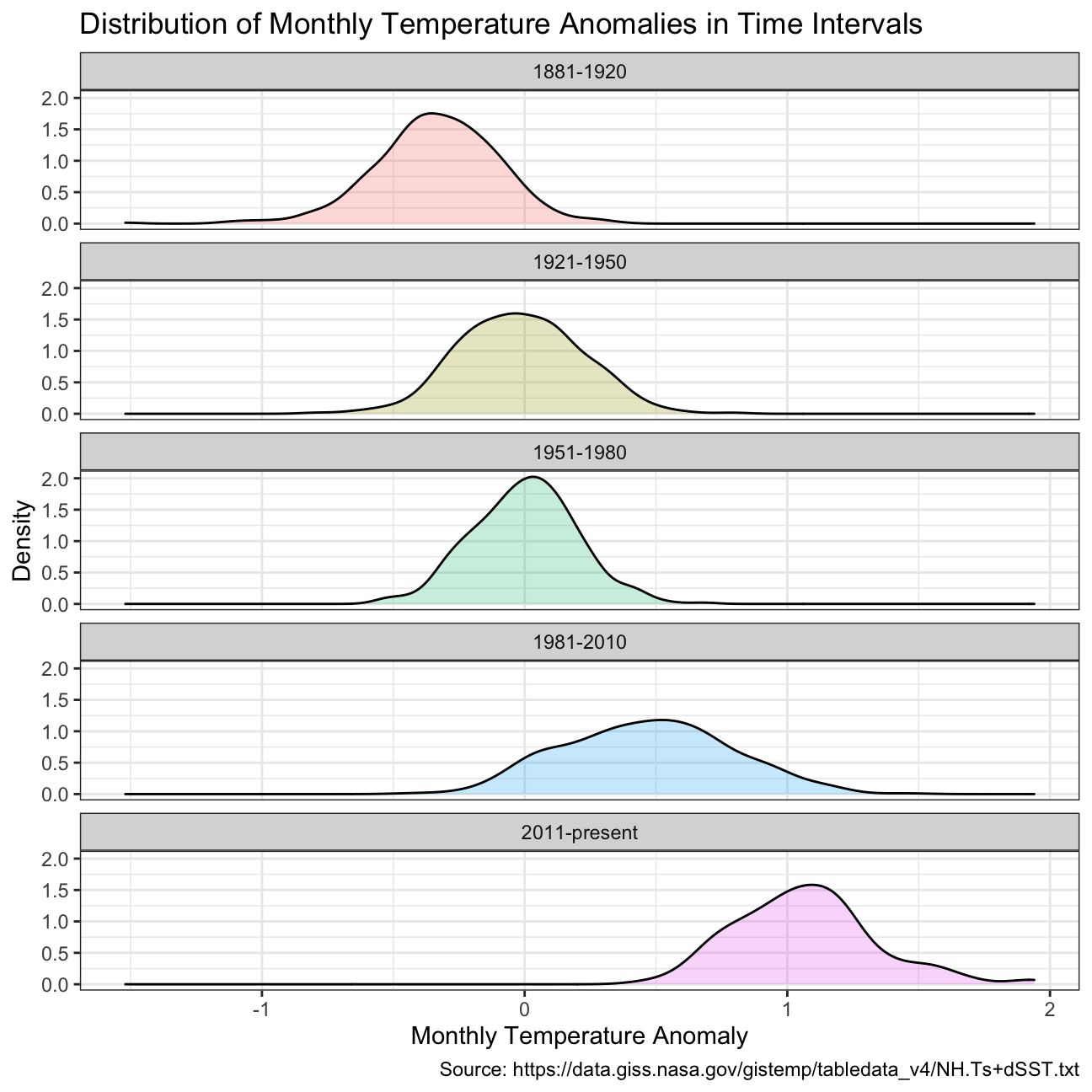

Calculating average annual anomalies.

#creating yearly averages
average_annual_anomaly <- tidyweather %>% 
  group_by(Year) %>%   #grouping data by Year
  
  # creating summaries for mean delta 
  summarise(mean_delta = mean(delta, na.rm=TRUE))

#plotting the data:

ggplot(average_annual_anomaly, 
       aes (x = Year,
            y = mean_delta)) +
  geom_point() +
  theme_bw() +
  geom_smooth(method = "loess") +
  labs(title = "Average annual anomalies by year",
       y = "Average annual anomalies",
    caption = "Source: https://data.giss.nasa.gov/gistemp/tabledata_v4/NH.Ts+dSST.txt") +
  NULL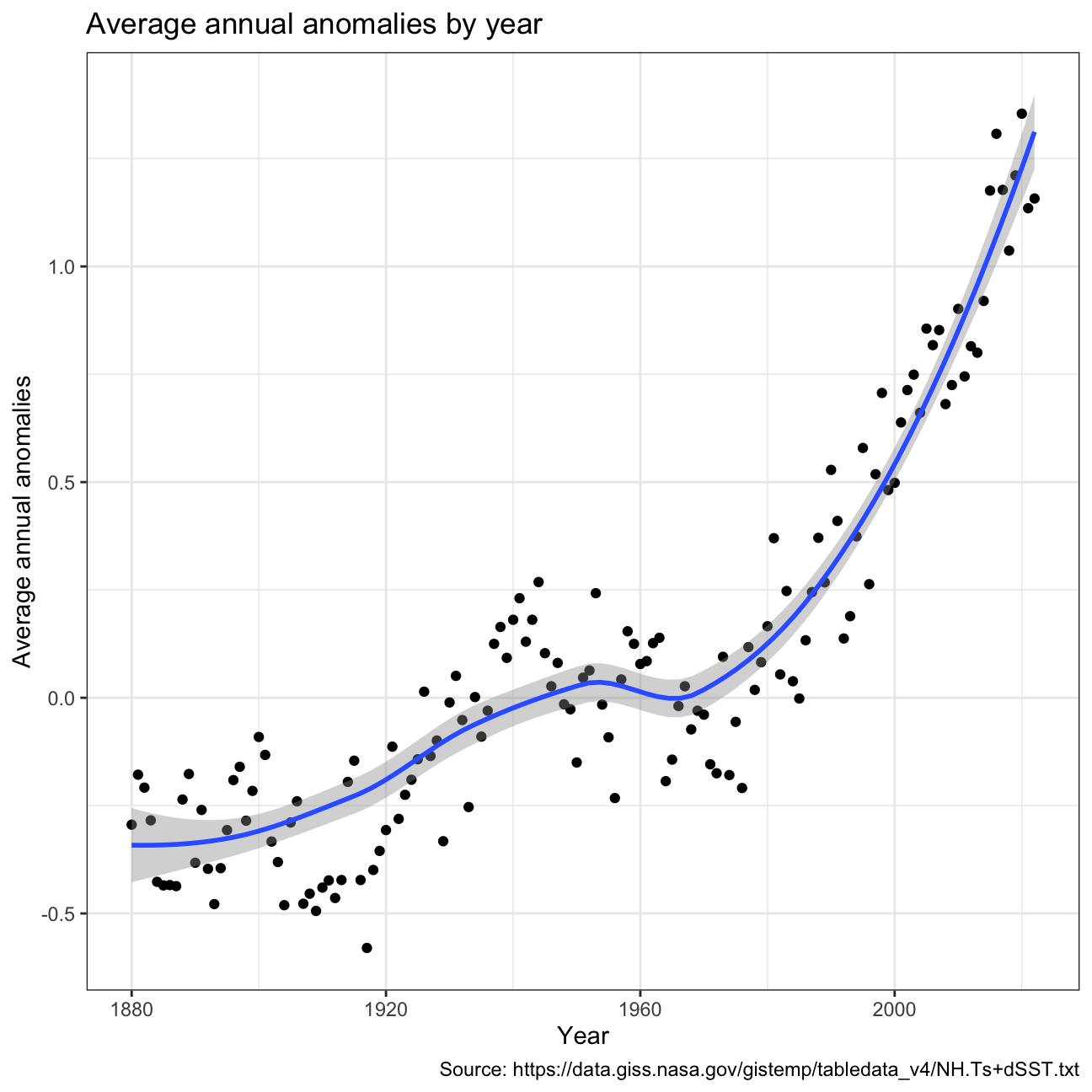

Confidence Interval for delta

NASA points out on their website that

A one-degree global change is significant because it takes a vast amount of heat to warm all the oceans, atmosphere, and land by that much. In the past, a one- to two-degree drop was all it took to plunge the Earth into the Little Ice Age.

Construction of a confidence interval for the average annual delta since 2011, both using a formula and using a bootstrap simulation with the infer package.

formula_ci <- comparison %>% 
  filter(interval == "2011-present") %>% # choose the interval 2011-present
  filter(!delta == "NA") %>% # drop NA observations in delta
  summarise(count = n(),
            t = qt(0.975, count-1), # use qt with probability and degrees of freedom
            mean = mean(delta), # calculate mean
            sd = sd(delta), # calculate sd
            se = sd(delta)/sqrt(count), # calculate se
            margin = t * se, # calculate margin of error
            lower = mean - margin, # calculate lower bound
            upper = mean + margin #calculate upper bound
            
  )

#print out formula_CI
formula_ci

## # A tibble: 1 × 8
##   count     t  mean    sd     se margin lower upper
##   <int> <dbl> <dbl> <dbl>  <dbl>  <dbl> <dbl> <dbl>
## 1   140  1.98  1.07 0.265 0.0224 0.0443  1.02  1.11

library(infer)

set.seed(1234)

boot_ci <- comparison %>% 
  filter(interval == "2011-present") %>% # choose the interval 2011-present
  filter(!delta == "NA") %>% # drop NA observations in delta
  specify(response = delta) %>% # specify the variable of interest
  generate(reps = 1000, type = "bootstrap") %>% # extract 1000 bootstrap samples
  calculate(stat = "mean") %>% # calculate sample means from each bootstrap sample
  get_confidence_interval(level = 0.95, type = "percentile") # calculate confidence interval of this analysis

# Display confidence interval
boot_ci

## # A tibble: 1 × 2
##   lower_ci upper_ci
##      <dbl>    <dbl>
## 1     1.02     1.11

Two different methods of constructing 95% confidence interval were used in this example. First was based on filtering appropriate interval and calculating confidence interval using summary statistics. Second involved ‘infer’ package, which allowed to use bootstrap method and produced the confidence intervals without any additional summary statistics. According to the summary calculations the average annual anomalies since 2011 already exceeded 1 degree, even when 95% confidence interval is taken into account. Therefore, it is highly likely that anomalies will become even more frequent and significant than before.